If you are subscribed to our mailing list this quote may sound familiar to you:
“Enhancements in this [DPL 9] release range from game-changing analytics to modeling ease-of-use to support for the latest technology platforms.”
When we said game-changing analytics we were, in large part, referring to the feature highlighted in this blog post: the ability to optimize multiple objective functions within a single DPL decision model. Needless to say, we’re thrilled to offer this new capability within the DPL 9 Enterprise version. Why? Because the Syncopation Team realizes that our more advanced user base are often confronted with decision-problems that include more than one objective or utility or criteria (or whatever you’d like to call it). In some situations, not all of the decisions are made by the same agent.
Talk about objectives, decisions, attributes and agents can be a bit abstract, so allow me to make it more clear by outlining the three levels of objective function difficulty:
Level 1 (least difficult)
There is one attribute (NPV ~= shareholder value) and the objective
function is crystal clear. The focus is on understanding the uncertainty
in your cash flows (which may not be crystal clear!).
“I’m a business manager and I need to decide which investment
alternative creates the most value.”
Level 2 (somewhat difficult)
There are multiple attributes and serious thought must be given to the
trade-offs among them in order to understand the objective function.
This level is where most multi-attribute decision analysis (MODA, MCDA,
MUA, MAU, etc.) takes place.
“I’m an environmental manager and I need to decide how to clean up this
contaminated site, trading off cost, public safety, worker safety and
environmental effects.”
Level 3 (most difficult)
There are multiple attributes and multiple, non-aligned decision makers
with different objective functions. This can range from relatively
friendly problems, such as joint venture partners with different
incentives, to purely adversarial problems, such as
counter-terrorism.
“I need to defend these key sites at minimal cost and disruption against
an adversary who just wants to kill as many people as possible.”
DPL has always been able to deal with Level 1 & 2 problems. Now, with DPL 9’s new multi-objective function capability in the DPL Enterprise version users will be able to tackle Level 3 problems, which are really a blend of decision analysis and game theory, in an intuitive and graphical decision tree environment.
There are a wide variety of these Level 3 problems that can be efficiently handled by DPL Enterprise. For example, on the one end you may have a joint venture partner that seeks to optimize a particular metric, e.g. total risk-adjusted sales of a pharmaceutical drug. But there may be a divergence in financial incentives due to the particulars of the deal, e.g., financial bonuses paid out for technical success at certain milestones. In this case both “agents” are on the same side – they’re working together to bring a new drug to market – but they have slightly different objectives. The problem discussed in detail below is at the other end of this spectrum:
DPL Multiple Objective Functions Case: Airport Defense
Imagine you are tasked with making a decision as to which, if any, airports to defend against attack in the US. Your alternatives are to defend none, the top 10, or the top 50. Your objective for the decision is to minimize fatalities and costs. While you’d like to defend all airports and incur no fatalities, that simply isn’t a feasible alternative in the real world. This situation could be modeled with a one up-front decision, a couple of attributes and a single objective function to be minimized that is the weighted sum of the attributes (fatalities & cost) as shown in the DPL input and output trees.
Note that the outcome of the Attack Airport chance node may be uncertain to you – but it’s really a decision that will be made by the attacker. Furthermore, underlying the Attacker’s decision are their own unique set of attribute weights which we do have some awareness of. To gain a fuller picture of the problem, we’re going to incorporate the attacker’s decision into the model, set up additional attributes that the attackers seek to optimize, and combine these into a second objective function for use in the model.
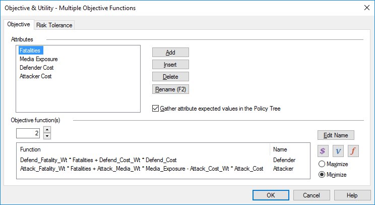
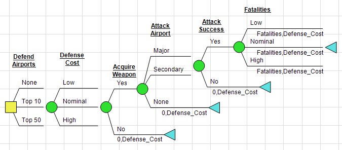
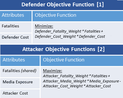
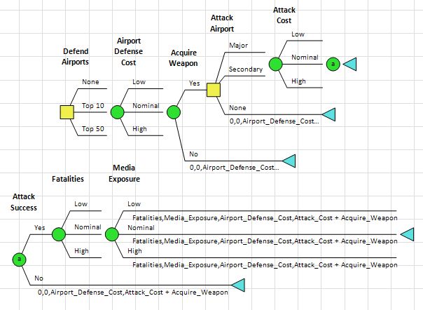
First you’ll change the Attack Airport chance node into a decision node. Next you’ll add a couple of nodes to the model for the Attacker’s attributes and weights. The table displays the attributes and objective function defined for the Defender and Attacker as specified within the DPL Objective & Utility dialog. You conferred with experts on the subject and came to the conclusion that the attacker is seeking to maximize both fatalities and media exposure while also minimizing cost. You’ll need to add a get/pay expression to the applicable branches in the decision tree for each attribute, which will result in the following Decision Tree:
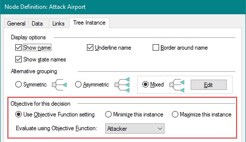
The last thing you’ll do to fully incorporate the second objective function for analysis is to tell DPL which of the two objective functions to use for each decision in the model. You can do this within the Node’s Definition on the Tree Instance tab:
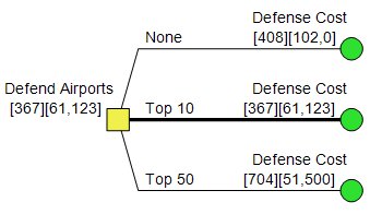
Now you can run an analysis on the model in order to generate results. As a part of a decision analysis run you can choose to generate risk profiles for each objective function and/or attribute defined in the model. Of most interest in this example is the Policy Tree:
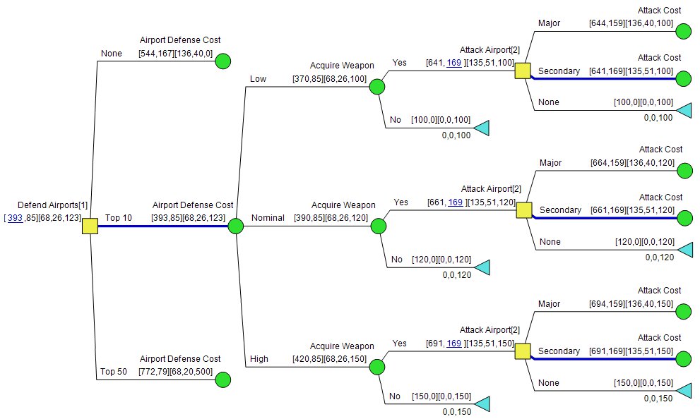
The Policy Tree tells you that the optimal decision policy is to still defend only the top 10 airports. Looking further down the tree, you’ll see that the Attacker’s optimal decision alternative is to attack a secondary location. You may be wondering about the blue lines and numbers. The blue shading indicates the optimal decision alternative (i.e., branch) and the Expected Value of the Objective Function used at that decision (as specified within the Tree Instance tab of the Node Definition dialog).
I hope you found this to be a useful introduction to this exciting, new DPL 9 Enterprise feature. If you’re interested in trying out the feature for yourself or simply discussing your multiple objective function problem, contact our team today.